Notes | Convex Optimization | Chapter4 Convex optimization problems

4.1 Optimization problems

4.1.1 Basic terminology

We use the notation

\[\begin{aligned} \text{minimize }\quad&f_0(x)\\\\ \text{subject to}\quad&f_i(x)\leq 0,\quad i=1,\dots,m\\\\ &h_i(x)=0,\quad i=1,\dots,p \tag{4.1} \end{aligned}\]

to describe the problem of finding an $x$ that minimizes $f_0(x)$ among all $x$ that satisfy the conditions $f_i(x)\leq 0,i=1,\dots,m$, and $h_i(x)=0,i=1,\dots,p$. We call $x\in\mathbf{R}^n$ the optimization variable and the function $f_0:\mathbf{R}^n\rightarrow\mathbf{R}$ the objective function or cost function. The inequalities $f_i(x)\leq 0$ are called inequality constraints, and the corresponding functions $f_i:\mathbf{R}^n\rightarrow\mathbf{R}$ are called the inequality constraint functions. The equations $h_i(x)=0$ are called the equality constraints, and the functions $h_i:\mathbf{R}^n\rightarrow\mathbf{R}$ are the equality constraint functions. If there are no constraints (i.e., $m=p=0$) we say the problem (4.1) is unconstrained.

The problem (4.1) is said to be feasible if there exists at least one feasible point, and infeasible otherwise. The set of all feasible points is called the feasible set or the constraint set.

The optimal value $p^*$ of the problem (4.1) is defined as

\[p^\*=\inf\\{f_0(x)|f_i(x)\leq 0,i=1,\dots,m,h_i(x)=0,i=1,\dots,p\\}\]

We allow $p^*$ to take on the extended values $\pm\infin$. If the problem is infeasible, we have $p^*=\infin$ (following the standard convention that the infimum of the empty set is $\infin$). If there are feasible points $x_k$ with $f_0(x_k)\rightarrow-\infin$ as $k\rightarrow\infin$, then $p^*\rightarrow-\infin$, and we say the problem (4.1) is unbounded below.

Optimal and locally optimal points:

We say a feasible point $x$ is locally optimal if there is an $R>0$ such that

\[f_0(x)=\inf\\{f_0(z)|f_i(z)\leq 0,i=1,\dots,m,h_i(z)=0,i=1,\dots,p,\lVert z-x\rVert_2\leq R\\},\]

with variable $z$. Roughly speaking, this means $x$ minimizes $f_0$ over nearby points in the feasible set.

Feasibility problems:

If the objective function is identically zero, the optimal value is either zero (if the feasible set is nonempty) or $\infin$ (if the feasible set is empty). We call this the feasibility problem, and will sometimes write it as

\[\begin{aligned} \text{find }\quad&x\\\\ \text{subject to}\quad&f_i(x)\leq 0,\quad i=1,\dots,m\\\\ &h_i(x)=0,\quad i=1,\dots,p. \end{aligned}\]

The feasibility problem is thus to determine whether the constraints are consistent, and if so, find a point that satisfies them.

4.1.2 Expressing problems in standard form

We refer to (4.1) as an optimization problem in standard form. In the standard form problem we adopt the convention that the righthand side of the inequality and equality constraints are zero.

Maximization problems:

We concentrate on the minimization problem by convention. We can solve the maximization problem

\[\begin{aligned} \text{maximize }\quad&f_0(x)\\\\ \text{subject to}\quad&f_i(x)\leq 0,\quad i=1,\dots,m\\\\ &h_i(x)=0,\quad i=1,\dots,p. \tag{4.2} \end{aligned}\]

by minimizing the function $-f_0$ subject to the constraints. By this correspondence we can define all the terms above for the maximization problem (4.2).

4.1.3 Equivalent problems

We call two problems equivalent if from a solution of one, a solution of the other is readily found, and vice versa.

We now describe some general transformations that yield equivalent problems.

Change of variables:

Suppose $\phi:\mathbf{R}^n\rightarrow\mathbf{R}^n$ is one-to-one, with image covering the problem domain $\mathcal{D}$, i.e., $\phi(\mathbf{dom}\phi)\supseteq\mathcal{D}$. We define functions $\tilde{f}_i$ and $\tilde{h}_i$ as

\[\tilde{f}_i=f_i(\phi(z)),i=0,\dots,m,\quad\tilde{h}_i(z)=h_i(\phi(z)),i=1,\dots,p.\]

Now consider the problem

\[\begin{aligned} \text{maximize }\quad&\tilde f_0(z)\\\\ \text{subject to}\quad&\tilde f_i(z)\leq 0,\quad i=1,\dots,m\\\\ &\tilde h_i(z)=0,\quad i=1,\dots,p. \tag{4.3} \end{aligned}\]

with variable $z$. We say that the standard form problem (4.1) and the problem (4.3) are related by the change of variable or substitution of variable $x=\phi(z)$.

Transformation of objective and constraint functions:

Suppose that $\psi_0:\mathbf{R}\rightarrow\mathbf{R}$ is monotone increasing, $\psi_1,\dots,\psi_m:\mathbf{R}\rightarrow\mathbf{R}$ satisfy $\psi_i(u)\leq 0$ if and only if $u\leq 0$, and $\psi_{m+1},\dots,\psi_{m+p}:\mathbf{R}\rightarrow\mathbf{R}$ satisfy $\psi_i(u)=0$ if and only if $u=0$. We define functions $\tilde f_i$ and $\tilde h_i$ as the compositions

\[\tilde f_i(x)=\psi_i(f_i(x)),\quad i=0,\dots,m,\qquad\tilde h_i(x)=\psi_{m+i}(h_i(x)),\quad i=1,\dots,p.\]

Evidently the associated problem

\[\begin{aligned} \text{minimize }\quad&\tilde f_0(x)\\\\ \text{subject to}\quad&\tilde f_i(x)\leq 0,\quad i=1,\dots,m\\\\ &\tilde h_i(x)=0,\quad i=1,\dots,p \end{aligned}\]

and the standard form problem (4.1) are equivalent; indeed, the feasible sets are identical, and the optimal points are identical.

Slack variables:

One simple transformation is based on the observation that $f_i(x)\leq 0$ if and only if there is an $s_i\geq 0$ that satisfies $f_i(x)+s_i=0$. Using this transformation we obtain the problem

\[\begin{aligned} \text{minimize }\quad&f_0(x)\\\\ \text{subject to}\quad&s_i\geq 0,\quad i=1,\dots,m\\\\ &f_i(x)+s_i=0,\quad i=1,\dots,m\\\\ &h_i(x)=0,\quad i=1,\dots,p, \end{aligned}\]

where the variables are $x\in\mathbf{R}^n$ and $s\in\mathbf{R}^m$. This problem has $n+m$ variables, $m$ inequality constraints (the nonnegativity constraints on $s_i$), and $m+p$ equality constraints. The new variable $s_i$ is called the slack variable associated with the original inequality constraint $f_i(x)\leq 0$.

Introducing slack variables replaces each inequality constraint with an equality constraint, and a nonnegativity constraint.

Eliminating equality constraints:

If we can explicitly parametrize all solutions of the equality constraints

\[h_i(x)=0,\quad i=1,\dots,p,\]

using some parameter $z\in\mathbf{R}^k$, then we can eliminate the equality constraints from the problem, as follows.

Eliminating linear equality constraints:

The process of eliminating variables can be described more explicitly, and easily carried out numerically, when the equality constraints are all linear, i.e., have the form $Ax=b$. If $Ax=b$ is inconsistent, i.e., $b\notin\mathcal{R}(A)$, then the original problem is infeasible. Assuming this is not the case, let $x_0$ denote any solution of the equality constraints. Let $F\in\mathbf{R}^{n\times k}$ be any matrix with $\mathcal{R}(F)=\mathcal{N}(A)$, so the general solution of the linear equations $Ax=b$ is given by $Fz+x_0$, where $z\in\mathbf{R}^k$.

Introducing equality constraints:

We can also introduce equality constraints and new variables into a problem.

Optimizing over some variables:

We always have

\[\inf_{x,y}f(x,y)=\inf_x\tilde f(x)\]

where $\tilde f(x)=\inf_yf(x,y)$. In other words, we can always minimize a function by first minimizing over some of the variables, and then minimizing over the remaining ones. This simple and general principle can be used to transform problems into equivalent forms.

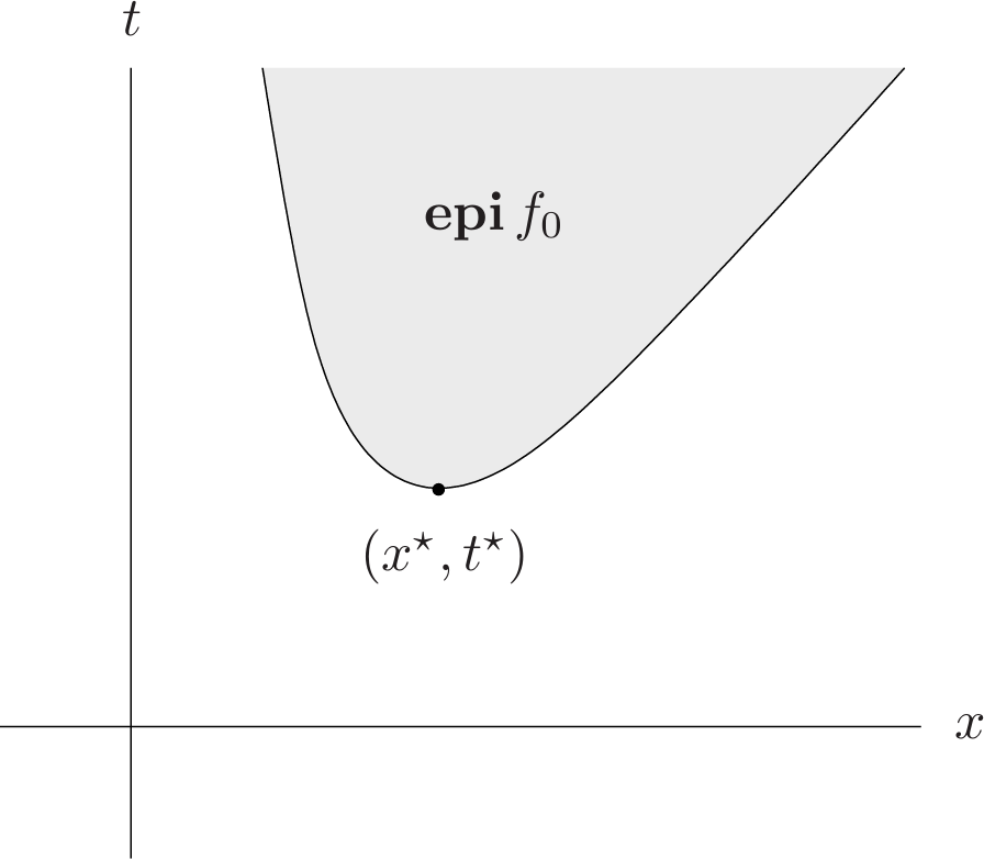
Epigraph problem form:

The epigraph form of the standard problem (4.1) is the problem

\[\begin{aligned} \text{minimize }\quad&t\\\\ \text{subject to}\quad&f_0(x)-t\leq 0\\\\ &f_i(x)\leq 0,\quad i=1,\dots,m\\\\ &h_i(x)=0,\quad i=1,\dots,p, \tag{4.4} \end{aligned}\]

with variable $x\in\mathbf{R}^n$ and $t\in\mathbf{R}$. We can easily see that it is equivalent to the original problem: $(x,t)$ is optimal for (4.4) if and only if $x$ is optimal for (4.1) and $t=f_0(x)$. Note that the objective function of the epigraph form problem is a linear function of the variables $x,t$.

Implicit and explicit constraints:

4.1.4 Parameter and oracle problem descriptions

In practice the distinction between a parameter and oracle problem description is not so sharp. If we are given a parameter problem description, we can construct an oracle for it, which simply evaluates the required functions and derivatives when queried. Most of the algorithms we study work with an oracle model, but can be made more efficient when they are restricted to solve a specific parametrized family of problems.

4.2 Convex optimization

4.2.1 Convex optimization problems in standard form

A convex optimization problem is one of the form

\[\begin{aligned} \text{minimize }\quad&f_0(x)\\\\ \text{subject to}\quad&f_i(x)\leq 0,\quad i=1,\dots,m\\\\ &a_i^Tx=b_i,\quad i=1,\dots,p, \tag{4.5} \end{aligned}\]

where $f_0,\dots,f_m$ are convex functions. Comparing (4.5) with the general standard form problem (4.1), the convex problem has three additional requirements:

• the objective function must be convex,
• the inequality constraint functions must be convex,
• the equality constraint functions $h_i(x)=a^T_ix−b_i$ must be affine.

In a convex optimization problem, we minimize a convex objective function over a convex set.

If $f_0$ is quasiconvex instead of convex, we say the problem (4.5) is a (standard form) quasiconvex optimization problem. Since the sublevel sets of a convex or quasiconvex function are convex, we conclude that for a convex or quasiconvex optimization problem the $\varepsilon$-suboptimal sets are convex. In particular, the optimal set is convex. If the objective is strictly convex, then the optimal set contains at most one point.

Concave maximization problems:

With a slight abuse of notation, we will also refer to

\[\begin{aligned} \text{maximize }\quad&f_0(x)\\\\ \text{subject to}\quad&f_i(x)\leq 0,\quad i=1,\dots,m\\\\ &a_i^Tx=b_i,\quad i=1,\dots,p, \tag{4.6} \end{aligned}\]

as a convex optimization problem if the objective function $f_0$ is concave, and the inequality constraint functions $f_1,\dots,f_m$ are convex.

Abstract form convex optimization problem:

Some authors use the term abstract convex optimization problem to describe the (abstract) problem of minimizing a convex function over a convex set.

4.2.2 Local and global optima

A fundamental property of convex optimization problems is that any locally optimal point is also (globally) optimal.

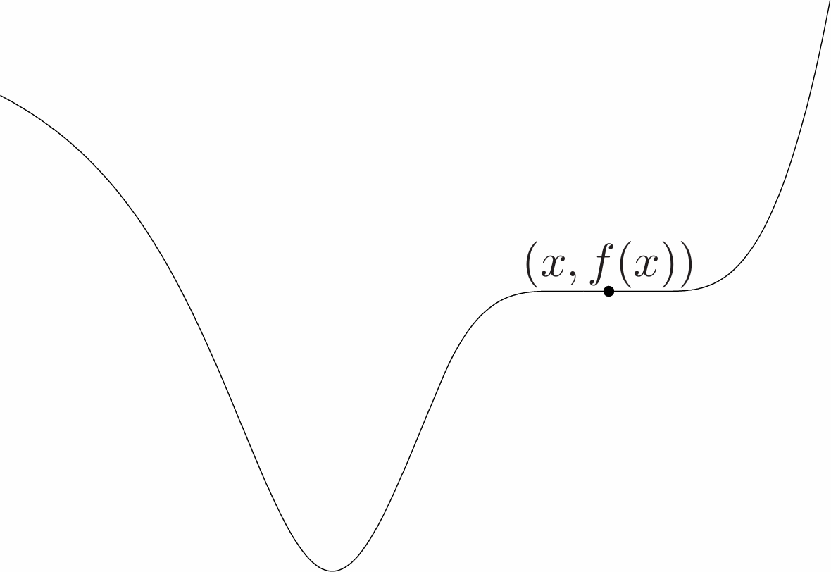
It is not true that locally optimal points of quasiconvex optimization problems are globally optimal.

4.2.3 An optimality criterion for differentiable $f_0$

Suppose that the objective $f_0$ in a convex optimization problem is differentiable, so that for all $x,y\in\mathbf{dom}f_0$,

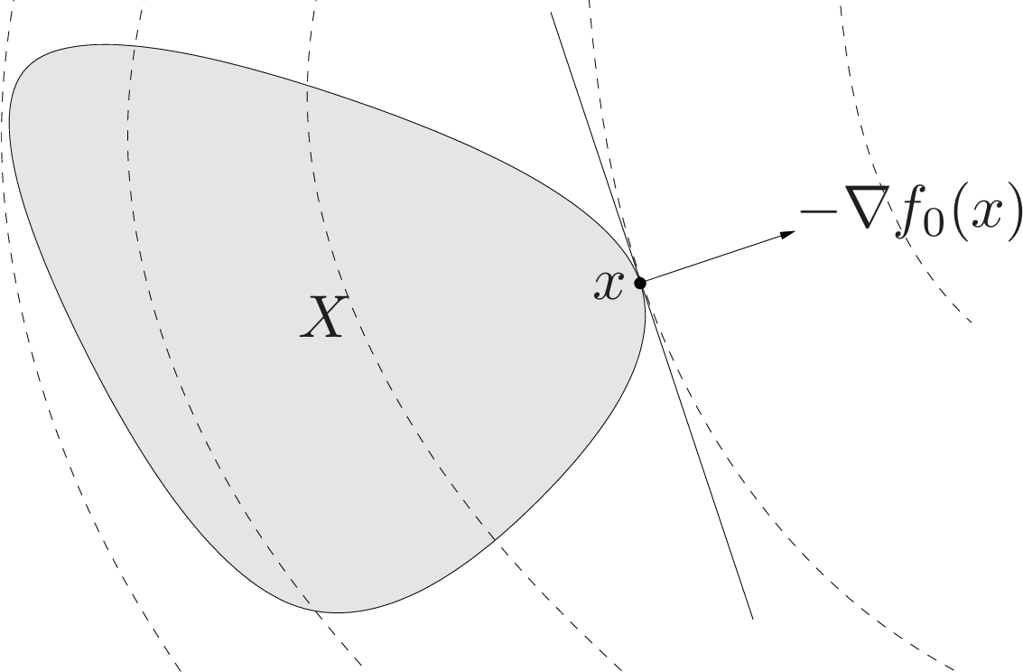
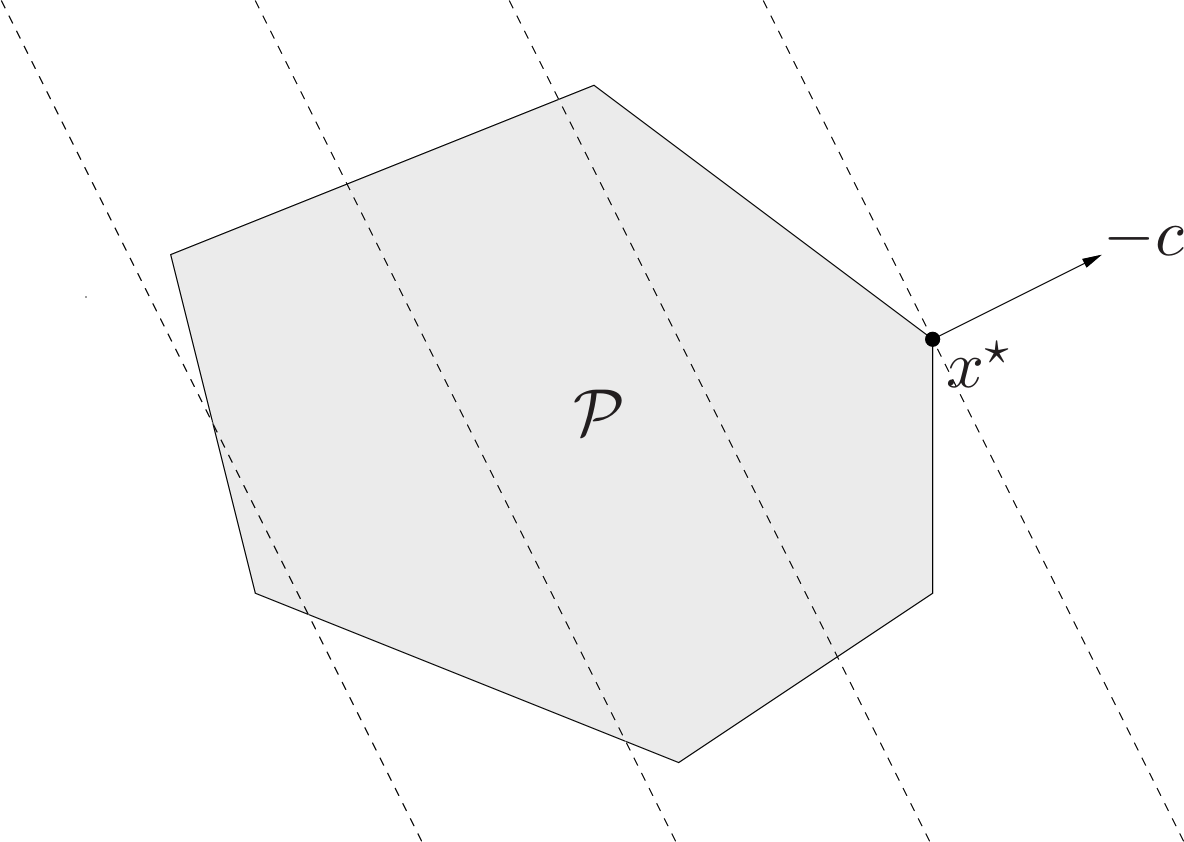
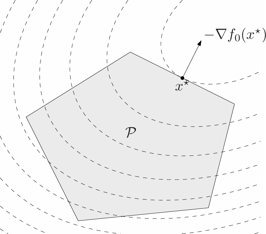
\[f_0(y)\geq f_0(x)+\nabla f_0(x)^T(y-x).\]

Let $X$ denote the feasible set, then $x$ is optimal if and only if $x\in X$ and

\[\nabla f_0(x)^T(y-x)\geq 0\text{ for all }y\in X. \tag{4.7}\]

This optimality criterion can be understood geometrically: If $\nabla f_0(x)\neq 0$, it means that $-\nabla f_0(x)$ defines a supporting hyperplane to the feasible set at $x$ (see Fig. 2.).

Problems with equality constraints only:

Consider the case where there are equality constraints but no inequality constraints, i.e.,

\[\begin{aligned} \text{maximize }\quad&f_0(x)\\\\ \text{subject to}\quad&Ax=b. \end{aligned}\]

Here the feasible set is affine. We assume that it is nonempty; otherwise the problem is infeasible. The optimality condition for a feasible $x$ is that

\[\nabla f_0(x)^T(y-x)\geq 0\]

must hold for all $y$ satisfying $Ay=b$. Since $x$ is feasible, every feasible $y$ has the form $y=x+v$ for some $v\in\mathcal{N}(A)$. The optimality condition can therefore be expressed as:

\[\nabla f_0(x)^Tv\geq 0\text{ for all }v\in\mathcal{N}(A).\]

If a linear function is nonnegative on a subspace, then it must be zero on the subspace, so it follows that $\nabla f_0(x)^Tv=0$ for all $v\in\mathcal{N}(A)$. In other words,

\[\nabla f_0(x)\perp\mathcal{N}(A).\]

Using the fact that $\mathcal{N}(A)^\perp=\mathcal{R}(A^T)$, this optimality condition can be expressed as $\nabla f_0(x)\in\mathcal{R}(A^T)$, i.e., there exists a $v\in\mathbf{R}^p$ such that

\[\nabla f_0(x)+A^Tv=0.\]

Together with the requirement $Ax=b$ (i.e., that $x$ is feasible), this is the classical Lagrange multiplier optimality condition.

4.2.4 Equivalent convex problems

Eliminating equality constraints:

At least in principle, we can restrict our attention to convex optimization problems which have no equality constraints. In many cases, however, it is better to retain the equality constraints, since eliminating them can make the problem harder to understand and analyze, or ruin the efficiency of an algorithm that solves it. This is true, for example, when the variable $x$ has very large dimension, and eliminating the equality constraints would destroy sparsity or some other useful structure of the problem.

Introducing equality constraints:

We can introduce new variables and equality constraints into a convex optimization problem, provided the equality constraints are linear, and the resulting problem will also be convex.

Slack variables:

By introducing slack variables we have the new constraints $f_i(x)+s_i=0$. Since equality constraint functions must be affine in a convex problem, we must have $f_i$ affine. In other words: introducing slack variables for linear inequalities preserves convexity of a problem.

Epigraph problem form:

The epigraph form of the convex optimization problem (4.5) is

\[\begin{aligned} \text{minimize }\quad&t\\\\ \text{subject to}\quad&f_0(x)-t\leq 0\\\\ &f_i(x)\leq 0,\quad i=1,\dots,m\\\\ &a_i^Tx=b_i,\quad i=1,\dots,p. \end{aligned}\]

The objective is linear (hence convex) and the new constraint function $f_0(x)−t$ is also convex in $(x,t)$, so the epigraph form problem is convex as well.

It is sometimes said that a linear objective is universal for convex optimization, since any convex optimization problem is readily transformed to one with linear objective.

Minimizing over some variables:

Minimizing a convex function over some variables preserves convexity.

4.2.5 Quasiconvex optimization

Recall that a quasiconvex optimization problem has the standard form

\[\begin{aligned} \text{minimize }\quad&f_0(x)\\\\ \text{subject to}\quad&f_i(x)\leq 0,\quad i=1,\dots,m\\\\ &Ax=b, \tag{4.8} \end{aligned}\]

where the inequality constraint functions $f_1,\dots,f_m$ are convex, and the objective $f_0$ is quasiconvex.

Locally optimal solutions and optimality conditions:

The most important difference between convex and quasiconvex optimization is that a quasiconvex optimization problem can have locally optimal solutions that are not (globally) optimal.

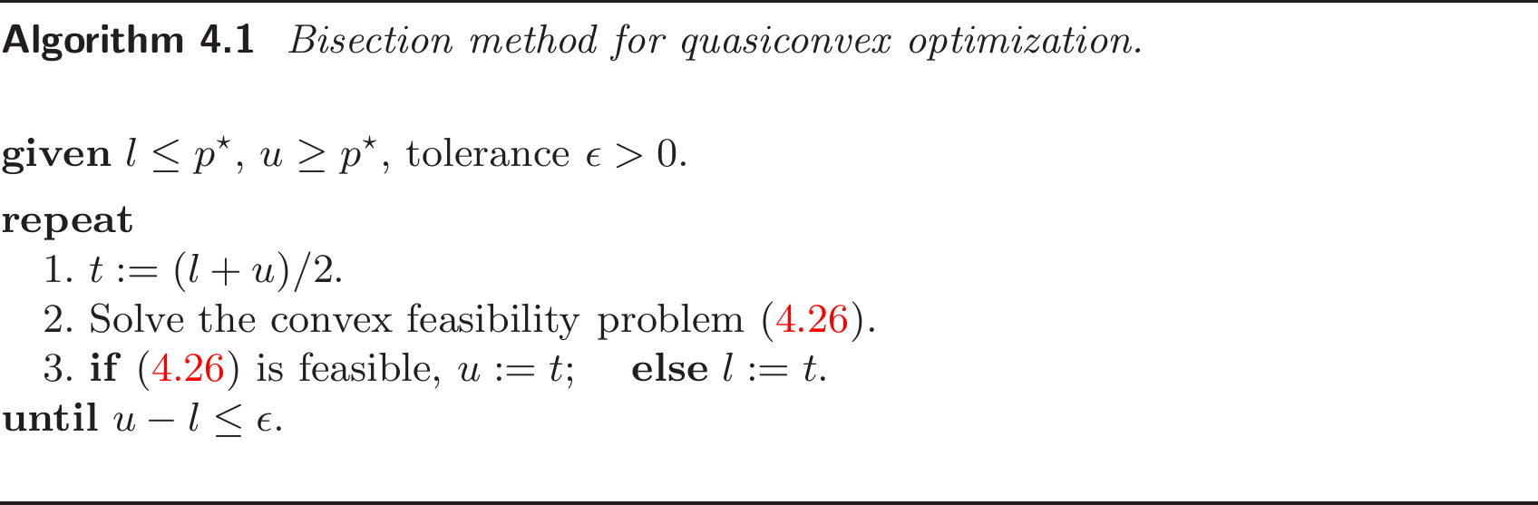
Quasiconvex optimization via convex feasibility problems:

Let $p^*$ donate the optimal value of the quasiconvex optimization problem (4.8). If the feasibility problem

\[\begin{aligned} \text{find }\quad&x\\\\ \text{subject to}\quad&\phi_t(x)\leq 0\\\\ &f_i(x)\leq 0,\quad i=1,\dots,m\\\\ &Ax=b, \tag{4.9} \end{aligned}\]

is feasible, then we have $p^*\leq t$. Conversely, if the problem (4.9) is infeasible, then we can conclude $p^*\geq t$.

This observation can be used as the basis of a simple algorithm for solving the quasiconvex optimization problem (4.8) using bisection, solving a convex feasibility problem at each step.

4.3 Linear optimization problems

When the objective and constraint functions are all affine, the problem is called a linear program (LP). A general linear program has the form

\[\begin{aligned} \text{minimize }\quad&c^Tx+d\\\\ \text{subject to}\quad&Gx\preceq h\\\\ &Ax=b, \tag{4.10} \end{aligned}\]

where $G\in\mathbf{R}^{m\times n}$ and $A\in\mathbf{R}^{p\times n}$. Linear programs are, of course, convex optimization problems.

Standard and inequality form linear programs:

Two special cases of the LP (4.10) are so widely encountered that they have been given separate names. In a standard form LP the only inequalities are componentwise nongativity constraints $x\succeq 0$:

\[\begin{aligned} \text{minimize }\quad&c^Tx\\\\ \text{subject to}\quad&Ax=b\\\\ &x\succeq 0. \tag{4.11} \end{aligned}\]

If the LP has no equality constraints, it is called an inequality form LP, usually written as

\[\begin{aligned} \text{minimize }\quad&c^Tx\\\\ \text{subject to}\quad&Ax\preceq b. \tag{4.12} \end{aligned}\]

Converting LPs to standard form:

It is sometimes useful to transform a general LP (4.10) to one in standard form (4.11). The first step is to introduce slack variables $s_i$ for the inequalities, which results in

\[\begin{aligned} \text{minimize }\quad&c^Tx+d\\\\ \text{subject to}\quad&Gx+s=h\\\\ &Ax=b\\\\ &s\succeq 0. \end{aligned}\]

The second step is to express the variable $x$ as the difference of two nonnegative variables $x^+$ and $x^-$, i.e., $x=x^+-x^-,x^+,x^-\succeq 0$. This yields the problem

\[\begin{aligned} \text{minimize }\quad&c^Tx^+-c^Tx^-+d\\\\ \text{subject to}\quad&Gx^+-Gx^-+s=h\\\\ &Ax^+-Ax^-=b\\\\ &x^+\succeq 0,\quad x^-\succeq 0,\quad s\succeq 0, \end{aligned}\]

which is an LP in standard form, with variable $x^+,x^-$, and $s$.

4.3.1 Examples

Chebyshev center of a polyhedron:

We consider the problem of finding the largest Euclidean ball that lies in a polyhedron described by linear inequalities,

\[\mathcal{P}=\\{x\in\mathbf{R}^n|a_i^Tx\leq b_i,i=1,\dots,m\\}.\]

The center of the optimal ball is called the Chebyshev center of the polyhedron; it is the point deepest inside the polyhedron, i.e., farthest from the boundary.

We present the ball as

\[\mathcal{B}=\\{x_c+u|\lVert u\rVert_2\leq r\\}.\]

The variables in the problem are the center $x_c\in\mathbf{R}^n$ and the radius $r$; we wish to maximize $r$ subject to the constraint $\mathcal{B}\subseteq\mathcal{P}$.

We start by considering the simpler constraint that $\mathcal{B}$ lies in one halfspace $a_i^Tx\leq b_i$, i.e.,

\[\lVert u\rVert_2\leq r\rightarrow a_i^T(x_c+u)\leq b_i. \tag{4.13}\]

Since

\[\sup\\{a_i^Tu|\lVert u\rVert_2\leq r\\}=r\lVert a_i\rVert_2\]

we can write (4.13) as

\[a_i^Tx_c+r\lVert a_i\rVert_2\leq b_i, \tag{4.14}\]

which is a linear inequality in $x_c$ and $r$. In other words, the constraint that the ball lies in the halfspace determined by the inequality $a_i^Tx\leq b_i$ can be written as a linear inequality.

Therefore $\mathcal{B}\subseteq\mathcal{P}$ if and only if (4.14) holds for all $i=1,\dots,m$. Hence the Chebyshev center can be determined by solving the LP

\[\begin{aligned} \text{maximize }\quad&r\\\\ \text{subject to}\quad&a_i^Tx_c+r\lVert a_i\rVert_2\leq b_i,\quad i=1,\dots,m, \end{aligned}\]

with variable $r$ and $x_c$.

4.3.2 Linear-fractional programming

The problem of minimizing a ratio of affine functions over a polyhedron is called a linear-fractional program:

\[\begin{aligned} \text{minimize }\quad&f_0(x)\\\\ \text{subject to}\quad&Gx\preceq h\\\\ &Ax=b \tag{4.15} \end{aligned}\]

where the objective function is given by

\[f_0(x)=\frac{c^Tx+d}{e^Tx+f},\quad\mathbf{dom}f_0=\\{x|e^Tx+f>0\\}.\]

The objective function is quasiconvex (in fact, quasilinear) so linear-fractional programs are quasiconvex optimization problems.

Transforming to a linear program:

If the feasible set is nonempty, the linear-fractional program (4.15) can be transformed to an equivalent linear program

\[\begin{aligned} \text{minimize }\quad&c^Ty+dz\\\\ \text{subject to}\quad&Gy-hz\preceq 0\\\\ &Ay-bz=0\\\\ e^Ty+fz=1\\\\ z\geq 0 \tag{4.16} \end{aligned}\]

with variable $y,z$.

To show the equivalence, we first note that if $x$ is feasible in (4.15) than the pair

\[y=\frac{x}{e^Tx+f},\quad z=\frac{1}{e^Tx+f}\]

is feasible in (4.16), with the same objective value $c^Ty+dz=f_0(x)$. It follows that the optimal value of (4.15) is greater than or equal to the optimal value of (4.16).

Generalized linear-fractional programming:

A generalization of the linear-fractional program (4.15) is the generalized linear-fractional program in which

\[f_0(x)=\max_{i=1,\dots,r}\frac{c_i^Tx+d_i}{e_i^Tx+f_i},\quad\mathbf{dom}f_0=\\{x|e_i^Tx+f_i>0,i=1,\dots,r\\}.\]

The objective function is the pointwise maximum of $r$ quasiconvex functions, and therefore quasiconvex, so this problem is quasiconvex. When $r=1$ it reduces to the standard linear-fractional program.

4.4 Quadratic optimization problems

The convex optimization problem (4.5) is called a quadratic program (QP) if the objective function is (convex) quadratic, and the constraint functions are affine. A quadratic program can be expressed in the form

\[\begin{aligned} \text{minimize }\quad&(1/2)x^TPx+q^Tx+r\\\\ \text{subject to}\quad&Gx\preceq h\\\\ &Ax=b, \tag{4.17} \end{aligned}\]

where $P\in\mathbf{S}_+^n,G\in\mathbf{R}^{m\times n}$, and $A\in\mathbf{R}^{p\times n}$.

4.4.1 Examples

Least-squares and regression:

The problem of minimizing the convex quadratic function

\[\lVert Ax-b\rVert _2^2=x^TA^TAx-2b^TAx+b^Tb\]

is an (unconstrained) QP. It arises in many fields and has many names, e.g., regression analysis or least-squares approximation. This problem is simple enough to have the well known analytical solution $x=A^\dag b$, where $A^\dag$ is the pseudo-inverse of $A$.

Distance between polyhedra:

The (Euclidean) distance between the polyhedra $\mathcal{P}_1=\{x

A_1x\preceq b_1\}$ and $\mathcal{P}_2=\{A_2x\preceq b_2\}$ in $\mathbf{R}^n$ is defined as

\[\mathbf{dist}(\mathcal{P}_1,\mathcal{P}_2)=\inf\\{\lVert x_1-x_2\rVert _2|x_1\in\mathcal{P}_1,x_2\in\mathcal{P}_2\\}.\]

If the polyhedra intersect, the distance is zero.

To find the distance between $\mathcal{P}_1$ and $\mathcal{P}_2$, we can solve the QP

\[\begin{aligned} \text{minimize }\quad&\lVert x_1-x_2\rVert _2^2\\\\ \text{subject to}\quad&A_1x_1\preceq b_1,\quad A_2x_2\preceq b_2, \end{aligned}\]

with variables $x_1,x_2\in\mathbf{R}^n$.

4.4.2 Second-order cone programming

A problem that is closely related to quadratic programming is the second-order cone program (SOCP):

\[\begin{aligned} \text{minimize }\quad&f^Tx\\\\ \text{subject to}\quad&\lVert A_ix+b_i\rVert _2\leq c_i^Tx+d_i,\quad i=1,\dots,m\\\\ &Fx=g, \tag{4.18} \end{aligned}\]

where $x\in\mathcal{R}^n$ is optimization variable, $A_i\in\mathbf{R}^{n_i\times n}$, and $F\in\mathbf{R}^{p\times n}$. We call constraint of the form

\[\lVert Ax+b\rVert _2\leq c^Tx+d,\]

where $A\in\mathbf{R}^{k\times n}$, a second-order cone constraint, since it is the same as requiring the affine function ($Ax+b,c^Tx+d$) to lie in the second-order cone in $\mathbf{R}^{k+1}$.

4.5 Geometric programming

In this section we describe a family of optimization problems that are not convex in their natural form. These problems can, however, be transformed to convex optimization problems, by a change of variables and a transformation of the objective and constraint functions

4.5.1 Monomials and posynomials

A function $f:\mathbf{R}^n\rightarrow\mathbf{R}$ with $\mathbf{dom}f=\mathbf{R}_{++}^n$, defined as

\[f(x)=cx_1^{a_1}x_2^{a_2}\cdots x_n^{a_n},\]

where $c>0$ and $a_i\in\mathbf{R}$, is called a monomial function, or simply, a monomial. A sum of monomials, i.e., a function of the form

\[f(x)=\sum_{k=1}^Kc_kx_1^{a_{1k}}x_2^{a_{2k}}\cdots x_n^{a_{nk}},\]

where $c_k>0$, is called a posynomial function (with $K$ terms), or simply, a posynomial.

4.5.2 Geometric programming

An optimization problem of the form

\[\begin{aligned} \text{minimize }\quad&f_0(x)\\\\ \text{subject to}\quad&f_i(x)\leq 1,\quad i=1,\dots,m\\\\ &h_i(x)=1,\quad i=1,\dots,p \tag{4.19} \end{aligned}\]

where $f_0,\dots,f_m$ are posynomials and $h_1,\dots,h_p$ are monomials, is called a geometric program (GP).

The domain of this problem is $\mathcal{D}=\mathcal{R}_{++}^n$; the constraint $x\succ 0$ is implicit.

4.5.3 Geometric program in convex form

Geometric programs are not (in general) convex optimization problems, but they can be transformed to convex problems by a change of variables and a transformation of the objective and constraint functions. The change of variables $y_i=\log x_i$ turns a monomial function into the exponential of an affine function. This results in the problem

\[\begin{aligned} \text{minimize }\quad&\tilde f_0(y)=\log(\sum_{k=1}^{K_0}e^{a_{0k}^Ty+b_{0k}})\\\\ \text{subject to}\quad&\tilde f_i(y)=\log(\sum_{k=1}^{K_i}e^{a_{ik}^Ty+b_{ik}})\leq 0,\quad i=1,\dots,m\\\\ &\tilde h_i(y)=g_i^Ty+hi=0,\quad i=1,\dots,p. \end{aligned}\]

Since the functions $\tilde f_i$ are convex, and $\tilde h_i$ are affine, the problem is a convex optimization problem. We refer to it as a geometric program in convex form. To distinguish it from the original geometric program, we refer to (4.19) as a geometric program in posynomial form.

4.6 Generalized inequality constraints

One very useful generalization of the standard form convex optimization problem (4.5) is obtained by allowing the inequality constraint functions to be vector valued, and using generalized inequalities in the constraints:

\[\begin{aligned} \text{minimize }\quad&f_0(x)\\\\ \text{subject to}\quad&f_i(x)\preceq_{K_i}0,\quad i=1,\dots,m\\\\ &Ax=b, \tag{4.20} \end{aligned}\]

where $f_0:\mathbf{R}^n\rightarrow\mathbf{R},K_i\subseteq\mathbf{R}^{k_i}$ are proper cones, and $f_i:\mathbf{R}^n\rightarrow\mathbf{R}^{k_i}$ are $K_i$-convex. We refer to this problem as a (standard form) convex optimization problem with generalized inequality constraints.

Many of the results for ordinary convex optimization problems hold for problems with generalized inequalities. Some examples are:

• The feasible set, any sublevel set, and the optimal set are convex.
• Any point that is locally optimal for the problem (4.20) is globally optimal.
• The optimality condition for differentiable $f_0$ holds without any change.

4.6.1 Conic form problems

Among the simplest convex optimization problems with generalized inequalities are the conic form problems (or cone programs), which have a linear objective and one inequality constraint function, which is affine (and therefore $K$-convex):

\[\begin{aligned} \text{minimize }\quad&c^Tx\\\\ \text{subject to}\quad&Fx+g\preceq_K0\\\\ &Ax=b. \end{aligned}\]

When $K$ is the nonnegative orthant, the conic form problem reduces to a linear program.

We can view conic form problems as a generalization of linear programs in which componentwise inequality is replaced with a generalized linear inequality.

Continuing the analogy to linear programming, we refer to the conic form problem

\[\begin{aligned} \text{minimize }\quad&c^Tx\\\\ \text{subject to}\quad&x\preceq_K0\\\\ &Ax=b \end{aligned}\]

as a conic form problem in standard form. Similarly, the problem

\[\begin{aligned} \text{minimize }\quad&c^Tx\\\\ \text{subject to}\quad&Fx+g\preceq_K0 \end{aligned}\]

is call a conic form problem in inequality form.

4.6.2 Semidefinite programming

When $K$ is $\mathbf{S}+^k$, the cone of positive semidefinite $k\times k$ matrices, the associated conic form problem is called a _semidefinite program (SDP), and has the form

\[\begin{aligned} \text{minimize }\quad&c^Tx\\\\ \text{subject to}\quad&x_1F_1+\cdots+x_nF_n+G\preceq0\\\\ &Ax=b, \end{aligned}\]

where $G,F_1,\dots,F_n\in\mathbf{S}^k$, and $A\in\mathbf{R}^{p\times n}$.

Standard and inequality form semidefinite programs:

Following the analogy to LP, a standard form SDP has linear equality constraints, and a (matrix) nonnegativity constraint on the variable $X\in\mathbf{S}^n$:

\[\begin{aligned} \text{minimize }\quad&\mathbf{tr}(CX)\\\\ \text{subject to}\quad&\mathbf{tr}(A_iX)=b_i,\quad i=1,\dots,p\\\\ &X\succeq 0, \end{aligned}\]

where $C,A_1,\dots,A_p\in\mathbf{S}^n$.

$\mathbf{tr}(CX)=\sum_{i,j=1}^nC_{ij}X_{ij}$ is the form of a general real-valued linear function on $\mathbf{S}^n$.

In LP and SDP standard forms, we minimize a linear function of the variable, subject to $p$ linear equality constraints on the variable, and a nonnegativity constraint on the variable.

An inequality form SDP, analogous to an inequality form LP (4.12), has no equality constraints, and one LMI:

\[\begin{aligned} \text{minimize }\quad&c^Tx\\\\ \text{subject to}\quad&x_1A_1+\cdots+x_nA_n\preceq B, \end{aligned}\]

with variable $x\in\mathbf{R}^n$, and parameters $B,A_1,\dots,A_n\in\mathbf{S}^k,c\in\mathbf{R}^n$.

4.6.3 Examples

Second-order cone programming:

The SOCP (4.18) can be expressed as a conic form problem

\[\begin{aligned} \text{minimize }\quad&c^Tx\\\\ \text{subject to}\quad&-(A_ix+b_i,c_i^Tx+d_i)\preceq_{K_i}0,\quad i=1,\dots,m\\\\ &Fx=g, \end{aligned}\]

in which

\[K_i=\\{(y,t)\in\mathbf{R}^{n_i+1}|\lVert y\rVert _2\leq t\\},\]

i.e., the second-order cone in $\mathbf{R}^{n_i+1}$. This explains the name second-order cone program for the optimization problem (4.18).

4.7 Vector optimization

4.7.1 General and convex vector optimization problems

In this section we investigate the meaning of a vector-valued objective function. We denote a general vector optimization problem as

\[\begin{aligned} \text{minimize (with respect to }K\text{) }\quad&f_0(x)\\\\ \text{subject to}\quad&f_i(x)\leq 0,\quad i=1,\dots,m\\\\ &h_i(x)=0,\quad i=1,\dots,p. \tag{4.21} \end{aligned}\]

Here $x\in\mathbf{R}^n$ is the optimization variable, $K\subseteq\mathbf{R}^q$ is a proper cone, $f_0:\mathbf{R}^n\rightarrow\mathbf{R}^q$ is the objective function, $f_i:\mathbf{R}^n\rightarrow\mathbf{R}$ are the inequality constraint functions, and $h_i:\mathbf{R}^n\rightarrow\mathbf{R}$ are the equality constraint functions.

In the context of vector optimization, the standard optimization problem (4.1) is sometimes called a scalar optimization problem.

We say the vector optimization problem (4.21) is a convex vector optimization problem if the objective function $f_0$ is $K$-convex, the inequality constraint functions $f_1,\dots,f_m$ are convex, and the equality constraint functions $h_1,\dots,h_p$ are affine.

4.7.2 Optimal points and values

We first consider a special case, in which the meaning of the vector optimization problem is clear. Consider the set of objective values of feasible points,

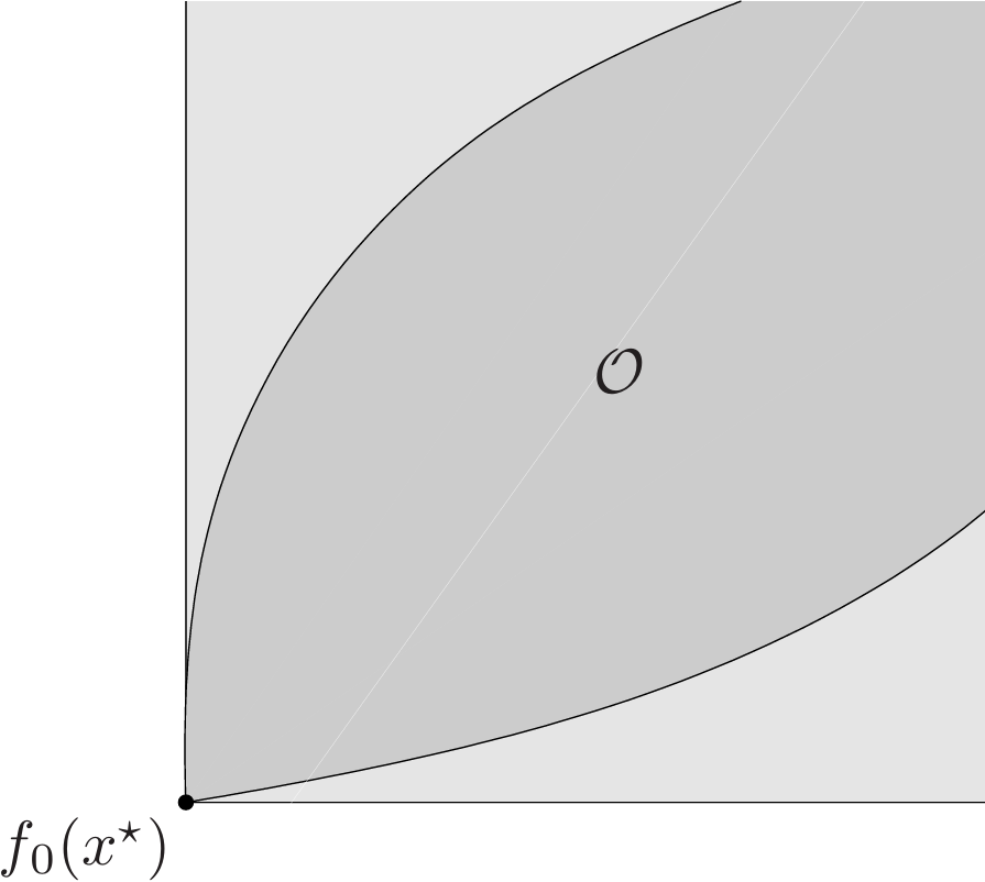
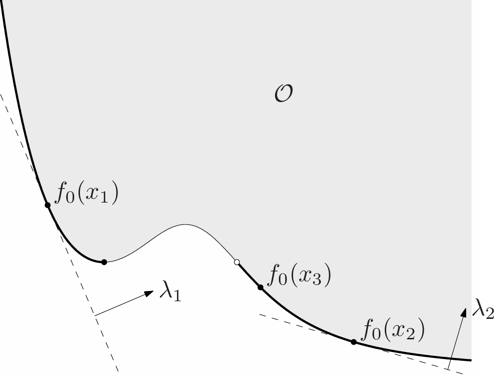
\[\mathcal{O}=\\{f_0(x)|\exist x\in\mathcal{D},f_i(x)\leq 0,i=1,\dots,m,h_i(x)=0,i=1,\dots,p\\}\subseteq\mathbf{R}^q,\]

which is called the set of achievable objective values. If this set has a minimum element, i.e., there is a feasible $x$ such that $f_0(x)\preceq_Kf_0(y)$ for all feasible $y$, then we say $x$ is optimal for the problem (4.21), and refer to $f_0(x)$ as the optimal value of the problem.

A point $x^*$ is optimal if and only if it is feasible and

\[\mathcal{O}\subseteq f_0(x^\*)+K \tag{4.22}\]

The set $f_0(x^*)+K$ can be interpreted as the set of values that are worse than, or equal to, $f_0(x^*)$, so the condition (4.22) states that every achievable value falls in this set.

Most vector optimization problems do not have an optimal point and an optimal value, but this does occur in some special cases.

4.7.3 Pareto optimal points and values

We say that a feasible point $x$ is Pareto optimal (or efficient) if $f_0(x)$ is a minimal element of the set of achievable values $\mathcal{O}$. In this case we say that $f_0(x)$ is a Pareto optimal value for the vector optimization problem (4.21).

A point $x$ is Pareto optimal if and only if it is feasible and

\[(f_0(x)-K)\cap\mathcal{O}=\\{f_0(x)\\} \tag{4.23}\]

The set $f_0(x)−K$ can be interpreted as the set of values that are better than or equal to $f_0(x)$, so the condition (4.23) states that the only achievable value better than or equal to $f_0(x)$ is $f_0(x)$ itself.

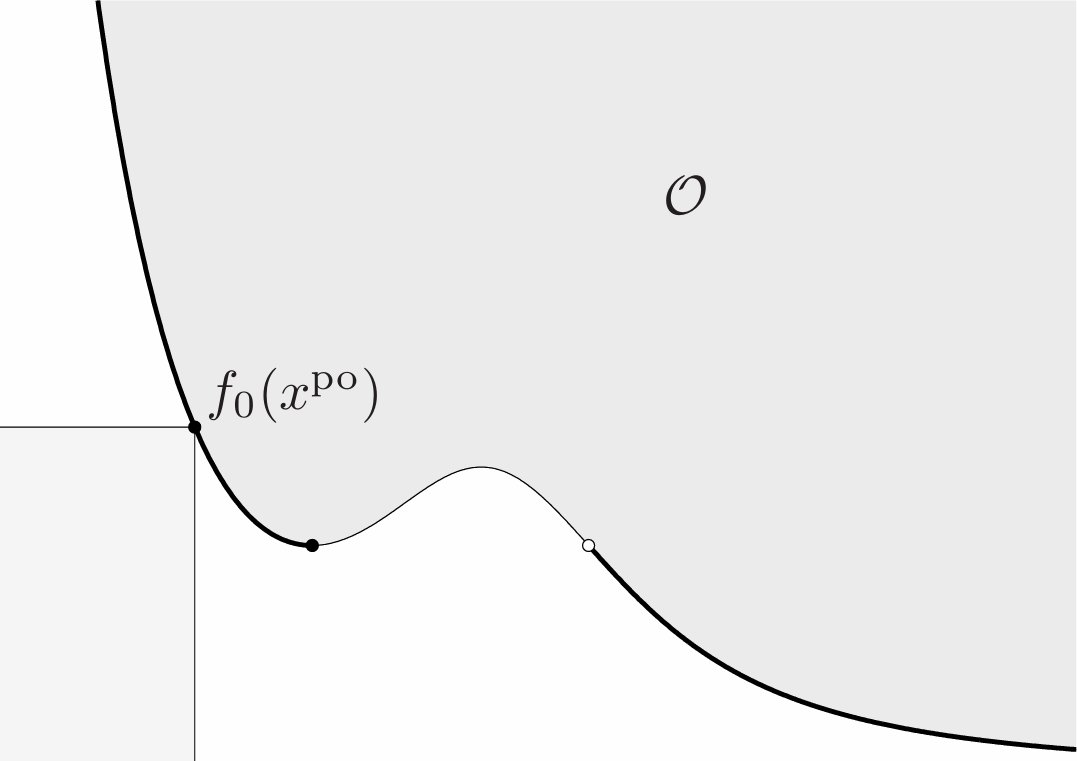
A vector optimization problem can have many Pareto optimal values (and points). The set of Pareto optimal values, denoted $\mathcal{P}$, satisfies

\[\mathcal{P}\subseteq\mathcal{O}\cap\mathbf{bd}\mathcal{O},\]

i.e., every Pareto optimal value is an achievable objective value that lies in the boundary of the set of achievable objective values.

4.7.4 Scalarization

Scalarization is a standard technique for finding Pareto optimal (or optimal) points for a vector optimization problem, based on the characterization of minimum and minimal points via dual generalized inequalities. Choose any $\lambda\succ_{K^*}0$, i.e., any vector that is positive in the dual generalized inequality. Now consider the scalar optimization problem

\[\begin{aligned} \text{minimize }\quad&\lambda^Tf_0(x)\\\\ \text{subject to}\quad&f_i(x)\leq 0,\quad i=1,\dots,m\\\\ &h_i(x)=0,\quad i=1,\dots,p, \tag{4.24} \end{aligned}\]

and let $x$ be the optimal point. Then $x$ is Pareto optimal for the vector optimization problem (4.21).

Using scalarization, we can find Pareto optimal points for any vector optimization problem by solving the ordinary scalar optimization problem (4.24).

The vector $\lambda$, which is sometimes called the weight vector, must satisfy $\lambda\succ_{K^*}$.

Scalarization of convex vector optimization problems:

Nowsuppose the vector optimization problem (4.21) is convex. Then the scalarized problem (4.24) is also convex, since $\lambda^Tf_0$ is a (scalar-valued) convex function. This means that we can find Pareto optimal points of a convex vector optimization problem by solving a convex scalar optimization problem. For each choice of the weight vector $\lambda\succ_{K^*}0$ we get a (usually different) Pareto optimal point.

We have to be careful here, because it is not true that every solution of the scalarized problem, with $\lambda\succeq_{K^*}0$ and $\lambda\neq 0$, is a Pareto optimal point for the vector problem. (In contrast, every solution of the scalarized problem with $\lambda\succ_{K^*}0$ is Pareto optimal.)

4.7.5 Multicriterion optimization

When a vector optimization problem involves the cone $K=\mathbf{R}+^q$, it is called a _multicriterion or multi-objective optimization problem. A multicriterion optimization problem is convex if $f_1,\dots,f_m$ are convex, $h_1,\dots,h_p$ are affine, and the objectives $F_1,\dots,F_q$ are convex.

If $x$ and $y$ are both feasible, we say that $x$ is better than $y$, or $x$ dominates $y$, if $F_i(x)_\leq F_i(y)$ for $i=1,dots,q$, and for at least one $j$, $F_j(x)<F_j(y)$.

In a multicriterion problem, an optimal point $x^*$ satisfies

\[F_i(x^\*)\leq F_i(y),\quad i=1,\dots,q,\]

for every feasible $y$. In other words, $x^*$ is simultaneously optimal for each of the scalar problems

\[\begin{aligned} \text{minimize }\quad&F_j(x)\\\\ \text{subject to}\quad&f_i(x)\leq 0,\quad i=1,\dots,m\\\\ &h_i(x)=0,\quad i=1,\dots,p, \end{aligned}\]

for $j=1,\dots,q$. When there is an optimal point, we say that the objectives are noncompeting, since no compromises have to be made among the objectives; each objective is as small as it could be made, even if the others were ignored.

Trade-off analysis:

When comparing two Pareto optimal points, they either obtain the same performance (i.e., all objectives equal), or, each beats the other in at least one objective.

Optimal trade-off analysis (or just trade-off analysis) is the study of how much worse we must do in one or more objectives in order to do better in some other objectives, or more generally, the study of what sets of objective values are achievable.

Optimal trade-off surface:

The set of Pareto optimal values for a multicriterion problem is called the optimal trade-off surface (in general, when $q>2$) or the optimal trade-off curve (when $q=2$).

Since it would be foolish to accept any point that is not Pareto optimal, we can restrict our trade-off analysis to Pareto optimal points.

Trade-off analysis is also sometimes called exploring the optimal trade-off surface.

An optimal trade-off curve is readily interpreted. An example is shown in Fig. 9, for a (convex) bi-criterion problem. From this curve we can easily visualize and understand the trade-offs between the two objectives.

• The endpoint at the right shows the smallest possible value of $F_2$, without any consideration of $F_1$.
• The endpoint at the left shows the smallest possible value of $F_1$, without any consideration of $F_2$.
• By finding the intersection of the curve with a vertical line at $F_1=\alpha$, we can see how large $F_2$ must be to achieve $F_1\leq\alpha$.
• By finding the intersection of the curve with a horizontal line at $F_2=\beta$, we can see how large $F_1$ must be to achieve $F_2\leq\beta$.
• The slope of the optimal trade-off curve at a point on the curve (i.e., a Pareto optimal value) shows the local optimal trade-off between the two objectives. Where the slope is steep, small changes in $F_1$ are accompanied by large changes in $F_2$.
• A point of large curvature is one where small decreases in one objective can only be accomplished by a large increase in the other. This is the proverbial knee of the trade-off curve, and in many applications represents a good compromise solution.

All of these have simple extensions to a trade-off surface, although visualizing a surface with more than three objectives is difficult.

Scalarizing multicriterion problems:

When we scalarize a multicriterion problem by forming the weighted sum objective

\[\lambda^Tf_0(x)=\sum_{i=1}^q\lambda_iF_i(x),\]

where $\lambda\succ 0$, we can interpret $\lambda_i$ as the weight we attach to the $i$thobjective. The weight $\lambda_i$ can be thought of as quantifying our desire to make $F_i$ small.