Notes | Convex Optimization | Chapter2 Convex sets

2.1 Affine and convex sets

2.1.1 Lines and line segments

Suppose $x_1\ne x_2$ are two points in ${\mathbf{R}}^n$. Points of the form

$$y=\theta x_1+(1-\theta )x_2$$

where $\theta \in \mathbf{R}$, form the line passing through $x_1$ and $x_2$. Expressing $y$ in the form

$$y=x_2+\theta (x_1-x_2)$$

gives another interpretation: $y$ is the sum of the base point $x_2$ (corresponding to $\theta =0$) and the direction $x_1-x_2$ (which points from $x_2$ to $x_1$) scaled by the parameter $\theta$.

2.1.2 Affine sets

A set $C\subseteq {\mathbf{R}}^n$ is affine if the line through any two distinct points in $C$ lies in $C$. We refer to a point of the form ${\theta }_1{x}_1+\cdots +{\theta }_k{x}_k$, where ${\theta }_1+\cdots +{\theta }_k=1$, as an affine combination of the points $x_1,\dots ,x_k$.

If $C$ is an affine set, $x_1,\dots ,x_k\in C$, and ${\theta }_1+\cdots +{\theta }_k=1$, then the point ${\theta }_1{x}_1+\cdots +{\theta }_k{x}_k$ also belongs to $C$.

If $C$ is an affine set and $x_0\in C$, then the set

$$\begin{gathered} V=C-x_0= \\ x-x_0|x\in C \end{gathered}$$

is a subspace. Suppose $v_1,v_2\in V$ and $\alpha ,\beta \in \mathbf{R}$. Then we have $v_1+x_0\in C$ and $v_2+x_0\in C$, and so

$$\alpha v_1+\beta v_2+x_0=\alpha (v_1+x_0)+\beta (v_2+x_0)+(1-\alpha -\beta )x_0\in C$$

since $C$ is affine, and $\alpha +\beta +(1-\alpha -\beta )=1$. we conclude that $\alpha v_1+\beta v_2\in V$, since $\alpha v_1+\beta v_2+x_0\in C$.

Thus, the affine set $C$ can be expressed as

$$\begin{gathered} C=V+x_0= \\ v+x_0|v\in V \end{gathered}$$

as a subspace plus an offset.

Every affine set can be expressed as the solution set of a system of linear equation. (See Example2.1)

The set of all affine combinations of points in some set $C\subseteq {\mathbf{R}}^n$ is called the affine hull if $C$, and denoted $\mathbf{aff}C$:

$$\begin{gathered} \mathbf{aff}C= \\ {\theta }_1{x}_1+\cdots +{\theta }_k{x}_k|x_1,\dots ,x_k\in C,{\theta }_1+\cdots +{\theta }_k=1 \end{gathered}$$

The affine hull is smallest affine set that contains $C$, in the following sense: if $S$ is any affine set with $C\subseteq S$, then $\mathbf{aff}C\subseteq S$

2.1.3 Affine dimension and relative interior

We define the affine dimension of a set $C$ as the dimension of its affine hull.

If the affine dimension of a set $C\subseteq {\mathbf{R}}^n$ is less than $n$, then the set lies in the affine set $\mathbf{aff}C\ne {\mathbf{R}}^n$. We define the relative interior of the set $C$, denoted $\mathbf{relint}C$ , as its interior relative to $\mathbf{aff}C$:

$$\begin{gathered} \mathbf{relint}C= \\ x\in C|B(x,r)\cap \mathbf{aff}C\subseteq C\text{ for some }r>0 \end{gathered}$$

where $B(x,r)=\{y

\lVert y-x\rVert\leq r\}$,theballofradius$r$andcenter$x$inthenorm$\lVert\cdot\rVert$. We can then define the relative boundary of a set $C$ as $\mathbf{cl}C\mathrm{\setminus }\mathbf{relint}C$, where $\mathbf{cl}C$ is the closure of $C$.

2.1.4 Convex sets

A set $C$ is convex if the line segment between any two point in $C$ lies in $C$. If for any $x_1,x_2\in C$ and any $\theta$ with $0\le \theta \le 1$, we have

$$\theta x_1+(1-\theta )x_2\in C$$

We call a point of the form ${\theta }_1{x}_1+\cdots +{\theta }_k{x}_k$, where ${\theta }_1+\cdots +{\theta }_k=1$ and ${\theta }_i\ge 0,i=1,\dots ,k$, a convex combination of the points $x_1,\dots ,x_k$. A convex combination of points can be thought of as a mixture or weighted average of the points, with ${\theta }_i$ the fraction of $x_i$ in the mixture.

The convex hull of a set $C$, denoted $\mathbf{conv}C$, is the set of all convex combinations of points in $C$:

$$\begin{gathered} \mathbf{conv}C= \\ {\theta }_1{x}_1+\cdots +{\theta }_k{x}_k|x_i\in C,{\theta }_i\ge 0,i=1,\dots ,k,{\theta }_1+\cdots +{\theta }_k=1 \end{gathered}$$

If $B$ is any convex set that contains $C$, then $\mathbf{conv}C\subseteq B$

2.1.5 Cones

A set $C$ is called a cone, or nonnegative homogeneous, if for every $x\in C$ and $\theta \ge 0$ we have $\theta x\in C$. A set $C$ is a convex cone if it is convex and a cone, which means that for any $x_1,x_2\in C$ and ${\theta }_1,{\theta }_2\ge 0$, we have

$${\theta }_1{x}_1+{\theta }_2{x}_2\in C$$

A point of the form ${\theta }_1{x}_1+\cdots +{\theta }_k{x}_k$ with ${\theta }_1,\dots ,{\theta }_k\ge 0$ is called a conic combination (or a nonnegative linear combination) of $x_1,\dots ,x_k$.

A set $C$ is a convex cone if and only if it contains all conic combinations of its elements.

The conic hull of a set $C$ is the set of all conic combinations of points in $C$

$${\theta }_1{x}_1\cdots +{\theta }_k{x}_k|x_i\in C,{\theta }_i\ge 0,i=1,\dots ,k$$

which is also the smallest convex cone that contains $C$

2.2 Some important examples

• The empty set $\mathrm{\varnothing }$, any single point (i.e., singleton) $\{x_0\}$, and the whole space ${\mathbf{R}}^n$ are affine (hence, convex) subsets of ${\mathbf{R}}^n$.
• Any line is affine. If it passes through zero, it is a subspace, hence also a convex cone.
• A line segment is convex, but not affine (unless it reduces to a point).

• A ray, which has the form $\{x_0 +\theta_v

  \theta\geq0\}$,where$v\neq0$,isconvex,butnotaffine.Itisaconvexconeifitsbase$x_0$ is 0.

• Any subspace is affine, and a convex cone (hence convex)

2.2.1 Hyperplanes and halfspaces

A hyperplane is as set of the form

$$x|a^{T}x=b$$

where $a\in {\mathbf{R}}^n,a\ne 0$, and $b\in \mathbf{R}$.

A hyperplane divides ${\mathbf{R}}^n$ into two halfspaces. A (closed) halfspace is a set of the form

$$x|a^{T}x\le b$$

where $a\ne 0$, the solution set of one (nontrivial) linear inequality.

Halfspaces are convex, but not affine.

The halfspace can also be expressed as

$$x|a^T(x-x_0)\le 0$$

where $x_0$ is any point on the associated hyperplane, satisfies $a^T{x}_0=b$.

The boundary of the halfspace is the hyperplane $\{x

a^Tx=b\}$.Theset$\{x

a^Tx<b\}$,whichistheinteriorofthehalfspace$\{x

a^Tx\leq b\}$, is called an open halfspace.

2.2.2 Euclidean balls and ellipsoids

A (Euclidean) ball (or just ball) in ${\mathbf{R}}^n$ has the form

$$\begin{gathered} B(x_c,r)= \\ x|\Vert x-x_c{\Vert }_2\le r \\ = \\ x|(x-x_c{)}^T(x-x_c)\le r^2 \end{gathered}$$

where $r>0$, and $\Vert \cdot {\Vert }_2$ denotes the Euclidean norm. The vector $x_c$ is the center of the ball and the scalar $r$ is its radius; $B(x_c,r)$ consists of all points within a distance r of center $x_c$. Another common representation for the Euclidean ball is

$$\begin{gathered} B(x_c,r)= \\ {x}_c+ru|\Vert u{\Vert }_2\le 1 \end{gathered}$$

A related family of convex sets is the ellipsoids, which have the form

$$\begin{gathered} \epsilon = \\ x|(x-x_c{)}^T{P}^{-1}(x-x_c)\le 1 \end{gathered}$$

where $P=P^T\succ 0$, $P$ is symmetric and positive definite. the vector $x_c\in {\mathbf{R}}^n$ is the center of the ellipsoid. The matrix $P$ determines how far the ellipsoid extends in every direction from $x_c$; the lengths of the semi-axes of $\epsilon$ are give by $\sqrt{{\lambda }_i}$, where ${\lambda }_i$ are the eigenvalue of $P$. A ball is an ellipsoid with $P=r^{2}I$.

Another common representation of an ellipsoid is

$$\begin{gathered} \epsilon = \\ {x}_c+Au|\Vert u{\Vert }_2\le 1 \end{gathered}$$

where A is square and nonsingular. In this representation we can assume without loss of generality that $A$ is symmetric and positive definite. When the matrix $A$ is symmetric positive semidefinite but singular, the set is called a degenerate ellipsoid; its affine dimension is equa to the rank of $A$. Degenerate ellipsoids are also convex.

2.2.3 Norm balls and norm cones

From the general properties of norms it can be shown that a norm ball of radius $r$ and center $x_c$, given by $\{x

\lVert x-x_c\rVert\leq r\}$ is convex. The norm cone associated with the norm $\Vert \cdot \Vert$ is the set

$$\begin{gathered} C= \\ (x,t)|\Vert x\Vert \le t \\ \subseteq {\mathbf{R}}^{n+1} \end{gathered}$$

It is (as the name suggests) a convex cone.

The second-order cone is the norm cone for the Euclidean norm,

$$\text{Missing left or extra right}$$

The second-order cone is also known by several other names. It is called the quadratic cone, since it is defined by a quadratic inequality. It is also called the Lorentz cone or ice-cream cone.

2.2.4 Polyhedra

A polyhedron is defined as the solution set of a finite number of line equalities and inequalities:

$$\begin{gathered} \mathcal{P}= \\ x|a_j^{T}x\le b_j,j=1,\dots ,m,c_j^{T}x=d_j,j=1,\dots ,p \end{gathered}$$

A polyhedron is thus the intersection of a finite number of halfspaces and hyperplanes.

Affine sets (e.g., subspaces, hyperplanes, lines), rays, line segments, and halfspaces are all polyhedra.

A bounded polyhedron is sometimes called a polytope, but sume authors use the opposite convention (i.e., polytope for any set of the preceding form, and polyhedron when it is bounded).

It will be convenient to use the compact notation

$$\begin{gathered} \mathcal{P}= \\ x|Ax⪯b,Cx=d \end{gathered}$$

where

$$A=\left[\begin{array}{c}{a}_1^T\\ \\ ⋮\\ \\ a_m^T\end{array}\right],C=\left[\begin{array}{c}{c}_1^T\\ \\ ⋮\\ \\ c_p^T\end{array}\right]$$

and the symbol $⪯$ denotes vector inequality or componentwise inequality in ${\mathbf{R}}^m$: $u⪯v$ means $u_i\le v_i$ for $i=1,\dots ,m$.

Simplexes:

Simplexes is another important family of polyhedra. Suppose the $k+1$ points $v_0,\dots ,v_k\in {\mathbf{R}}^n$ are affinely independent, which means $v_1-v_0,\dots ,v_k-v_0$ are linearly independent. The simplex determined by them is given by

$$\begin{gathered} C=\mathbf{conv} \\ {v}_0,\dots ,v_k \\ = \\ {\theta }_0{v}_0+\cdots +{\theta }_k{v}_k|\theta ⪯0,{\mathbf{1}}^T\theta =1 \end{gathered}$$

The affine dimension of this simplex is $k$, so it is sometimes referred to as a k-dimensional simplex in ${\mathbf{R}}^n$.

Some common simplexes. A 1-dimensional simplex is a line segment; a 2-dimensional simplex is a triangle (including its interior); and a 3-dimensional simplex is a tetrahedron.

Convex hull description of polyhedra:

The convex hull of the finite set $\{v_1,\dots ,v_k\}$ is

$$\begin{gathered} \mathbf{conv} \\ {v}_1,\dots ,v_k \\ = \\ {\theta }_1{v}_1+\cdots +{\theta }_k{v}_k|\theta ⪯0,{\mathbf{1}}^T\theta =1 \end{gathered}$$

This set is a polyhedron, and bounded, but (except is special cases, e.g., a simplex) it is not simple to express it in the form by a set of linear equalities and inequalities.

2.2.5 The positive semidefinite cone

We use the notation ${\mathbf{S}}^n$ to denote the set of symmetric $n\times n$ matrices,

$$\begin{gathered} {\mathbf{S}}^n= \\ X\in {\mathbf{R}}^{n\times n}|X=X^T \end{gathered}$$

which is a vector space with dimension $n(n+1)/2$. We use the notation ${\mathbf{S}}_{+}^n$ to denote the set of symmetric positive semidefinite matrices:

$$\begin{gathered} {\mathbf{S}}_{+}^n= \\ X\in {\mathbf{S}}^n|X⪰0 \end{gathered}$$

and the notation ${\mathbf{S}}_{++}^n$ to denote the set of symmetric positive definite matrices:

$$\begin{gathered} {\mathbf{S}}_{++}^n= \\ X\in {\mathbf{S}}^n|X\succ 0 \end{gathered}$$

The set ${\mathbf{S}}_{+}^n$ is a convex cone: if ${\theta }_1,{\theta }_2\ge 0$ and $A,B\in {\mathbf{S}}_{+}^n$, then ${\theta }_{1}A+{\theta }_{2}B\in {\mathbf{S}}_{+}^n$. This can be seen directly from the definition of positive semidefiniteness: for any $x\in {\mathbf{R}}^n$, we have

$$x^T({\theta }_{1}A+{\theta }_{2}B)x={\theta }_1{x}^{T}Ax+{\theta }_2{x}^{T}Bx\ge 0$$

if $A⪰0,B⪰0$ and ${\theta }_1,{\theta }_2\ge 0$.

2.3 Operations that preserve convexity

2.3.1 Intersection

Convexity is preserved under intersection: if $S_1$ and $S_2$ are convex, then $S_1\cap S_2$ is convex. This property extends to the intersection of an infinite number of sets: if $S_{\alpha }$ is convex for every $\alpha \in \mathbf{A}$, then $\bigcap _{\alpha \in \mathbf{A}}{S}_{\alpha }$ is convex.

every closed convex set $S$ is a (usually infinite) intersection of halfspaces. In fact, a closed convex set $S$ is the intersection of all halfspaces that contain it:

$$\begin{gathered} S=\bigcap \\ \mathcal{H}|\mathcal{H}\text{halfspace},S\subseteq \mathcal{H} \end{gathered}$$

2.3.2 Affine functions

Recall that a function $f:{\mathbf{R}}^n\leftarrow {\mathbf{R}}^m$ is affine if it is a sum of a linear function and a constant, i.e., if it has the form $f(x)=Ax+b$, where $A\in {\mathbf{R}}^{m\times n}$ and $b\in {\mathbf{R}}^m$. Suppose $S\subseteq {\mathbf{R}}^n$ is convex and $f:{\mathbf{R}}^n\leftarrow {\mathbf{R}}^m$ is an affine function. Then the image of $S$ under $f$,

$$\begin{gathered} f(S)= \\ f(x)|x\in S \end{gathered}$$

is convex.

2.3.3 Linear-fractional and perspective functions

The perspective function:

We define the perspective function $P:{\mathbf{R}}^{n+1}\to {\mathbf{R}}^n$, with domain $\mathbf{dom}P={\mathbf{R}}^n\times {\mathbf{R}}_{++}$, as $P(z,t)=z/t$. The perspective function scales or normalizes vectors so the last component is one, and then drops the last component

Remark. We can interpret the perspective function as the action of a pin-hole camera.

Linear-fractional functions:

A linear-fractional function is formed by composing the perspective function with an affine function. Suppose $g:{\mathbf{R}}^n\to {\mathbf{R}}^{m+1}$ is affine, i.e.,

$$g(x)=\left[\begin{array}{c}A\\ \\ c^T\end{array}\right]x+\left[\begin{array}{c}b\\ \\ d\end{array}\right]$$

where $A\in {\mathbf{R}}^{m\times n},b\in {\mathbf{R}}^m,c\in {\mathbf{R}}^n$, and $d\in \mathbf{R}$. The function $f:{\mathbf{R}}^n\to {\mathbf{R}}^m$ given by $f=P\circ g$, i.e.,

$$\begin{gathered} f(x)=(Ax+b)/(c^{T}x+d),\mathbf{dom}f= \\ x|c^{T}x+d>0 \end{gathered}$$

is called a linear-fractional (or projective) function. If $c=0$ and $d>0$, the domain of $f$ is ${\mathbf{R}}^n$, and $f$ is an affine function. So we can think of affine and linear functions as special cases of linear-fractional functions.

2.4 Generalized inequalities

2.4.1 Proper cones and generalized inequalities

A cone $K\subseteq {\mathbf{R}}^n$ is called a proper cone if it satisfies the followings:

• $K$ is convex.
• $K$ is closed.
• $K$ is solid, which means it has nonempty interior.
• $K$ is pointed, which means that it contains no line (or equivalently, $x\in K,-x\in K\Rightarrow x=0$)

A proper cone $K$ can be used to define a generalized inequality, which is a partial ordering on ${\mathbf{R}}^n$ that has many of the properties of the standard ordering on $\mathbf{R}$.

Cone of polynomials nonnegative on $[0,1]$. Let $K$ be defined as

$$\begin{gathered} K= \\ c\in {\mathbf{R}}^n|c_1+c_{2}t+\cdots +c_n{t}^{n-1}\ge 0\text{ for }t\in [0,1] \end{gathered}$$

i.e., $K$ is the cone of (coefficients of) polynomials of degree $n-1$ that are nonnegative on the interval $[0,1]$.

Properties of generalized inequalities:

A generalized inequality ${⪯}_K$ satisfies many properties, such as

• $\preceq K$ _is preserved under addition: if $x{⪯}_{K}y$ and $y{⪯}_{K}v$, then $x+u{⪯}_{K}y+v$.
• $\preceq K$ _is transitive: if $x{⪯}_{K}y$ and $y{⪯}_{K}z$, then $x{⪯}_{K}z$.
• $\preceq K$ _is preserved under nonnegative scaling: if $x{⪯}_{K}y$ and $\alpha \ge 0$, then $\alpha x{⪯}_K\alpha y$.
• $\preceq K$ _is reflexive: $x{⪯}_{K}x$.
• $\preceq K$ _is antisymmetric: if $x{⪯}_{K}y$ and $y{⪯}_{K}x$, then $x=y$.
• $\preceq K$ _is preserved under limits: if $x_i{⪯}_K{y}_i$ for $i=1,2,\dots ,x_i\to x$ and $y_i\to y$ as $i\to \text{infin}$, then $x{⪯}_{K}y$.

The correspoinding strict generalized inequality ${\prec }_K$ satisfies, for example,

• if $x{\prec }_{K}y$ then $x{⪯}_{K}y$.
• if $x{\prec }_{K}y$ and $u{⪯}_{K}v$ then $x+u{\prec }_{K}y+v$.
• if $x{\prec }_{K}y$ and $\alpha >0$ then $\alpha x{\prec }_K\alpha y$.
• $x{\nprec }_{K}x$.
• if $x{\prec }_{K}y$, then for $u$ and $v$ small enough, $x+u{⪯}_{K}y+v$.

2.4.2 Minimum and minimal elements

The most difference is that $\le$ on $\mathbf{R}$ is a linear ordering: any two points are comparable, meaning either $x\le y$ or $y\le x$. This property does not hold for other generalized inequalities. One implication is that concepts like minimum and maximum are more complicated in the context of generalized inequalities.

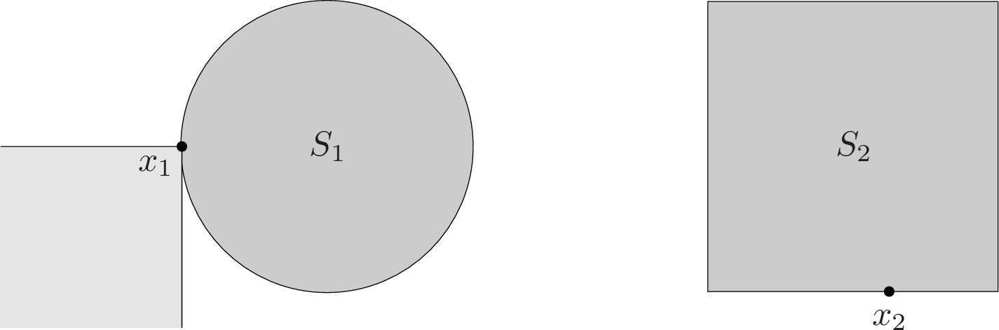
We can describe minimum and minimal elements using simple set notation. A point $x\in S$ is the minimum element of $S$ if and only if

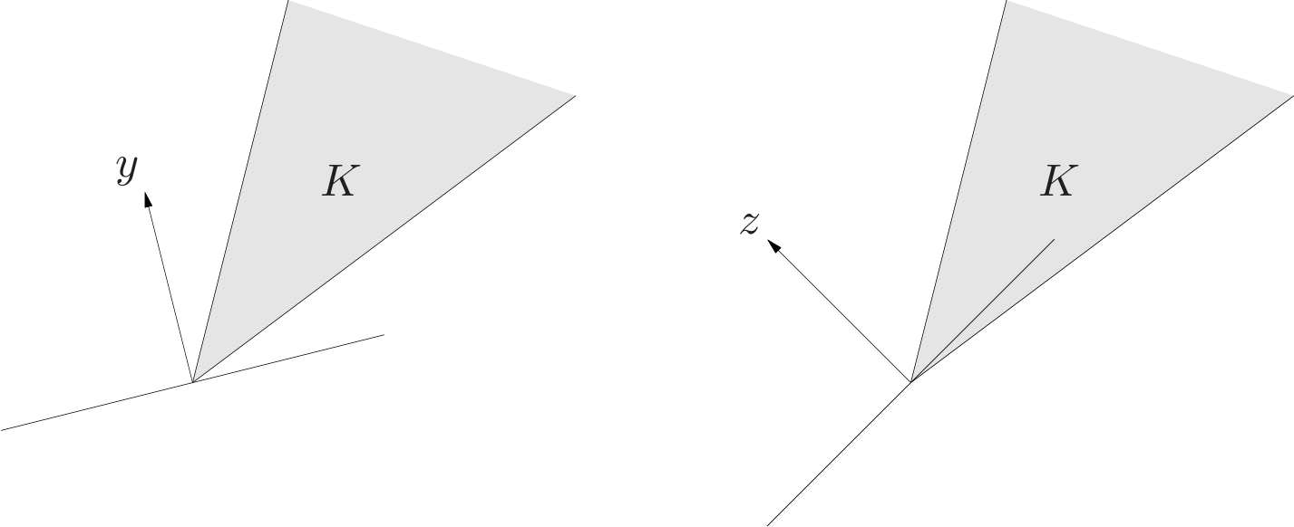
$$S\subseteq x+K$$

Here $x+K$ denotes all the points that are comparable to $x$ and greater than or equal to $x$ (according to ${⪯}_K$). A point $x\in S$ is a minimal element if and only if

$$\begin{gathered} (x-K)\cap S= \\ x \end{gathered}$$

Here $x-K$ denotes all the points that are comparable to $x$ and less than or equal to $x$ (according to ${⪯}_K$); the only point in common with $S$ is $x$.

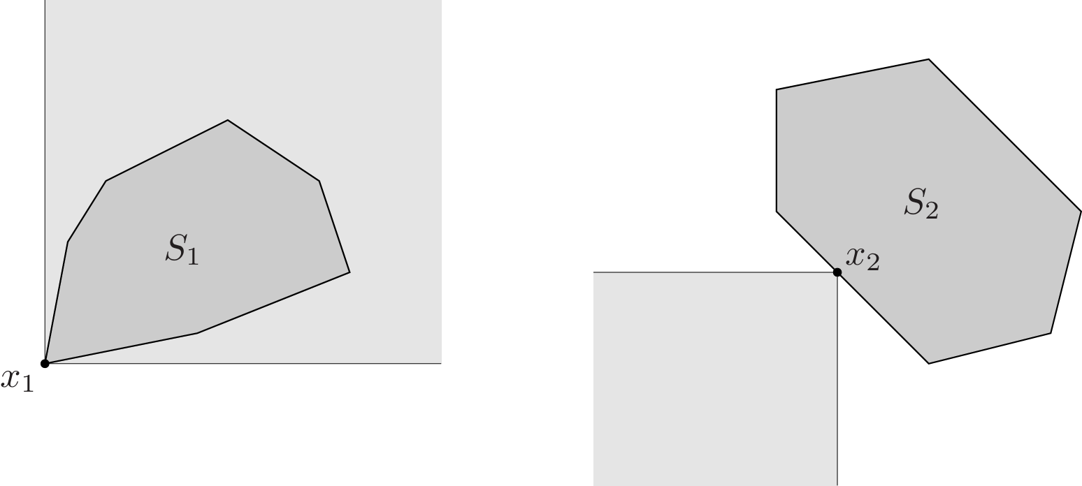
• Left. The set $S_1$ has a minimum element $x_1$ with respect to componentwise inequality in ${\mathbf{R}}^2$. The set $x_1+K$ is shaded lightly; $x_1$ is the minimum element of $S_1$ since $S_1\subseteq x_1+K$.
• Right. The point $x_2$ is a minimal point of $S_2$. The set $x_2-K$ is shown lightly shaded. The point $x_2$ is minimal because $x_2-K$ and $S_2$ intersect only at $x_2$.

2.5 Separating and supporting hyperplanes

2.5.1 Separating hyperplane theorem

separating hyperplane theorem: Suppose $C$ and $D$ are nonempty disjoint convex sets, i.e., $C\cap D=\mathrm{\varnothing }$. Then there exist $a\ne 0$ and $b$ such that $a^{T}x\le b$ for all $x\in C$ and $a^{T}x\ge b$ for all $x\in D$.In other words, the affine function $a^{T}x-b$ is nonpositive on $C$ and nonnegative on $D$. The hyperplane $\{x

a^Tx=b\}$ is call a separating hyperplane for the sets $C$ and $D$, or is said to separate the sets $C$ and $D$.

Proof of separating hyperplane theorem:

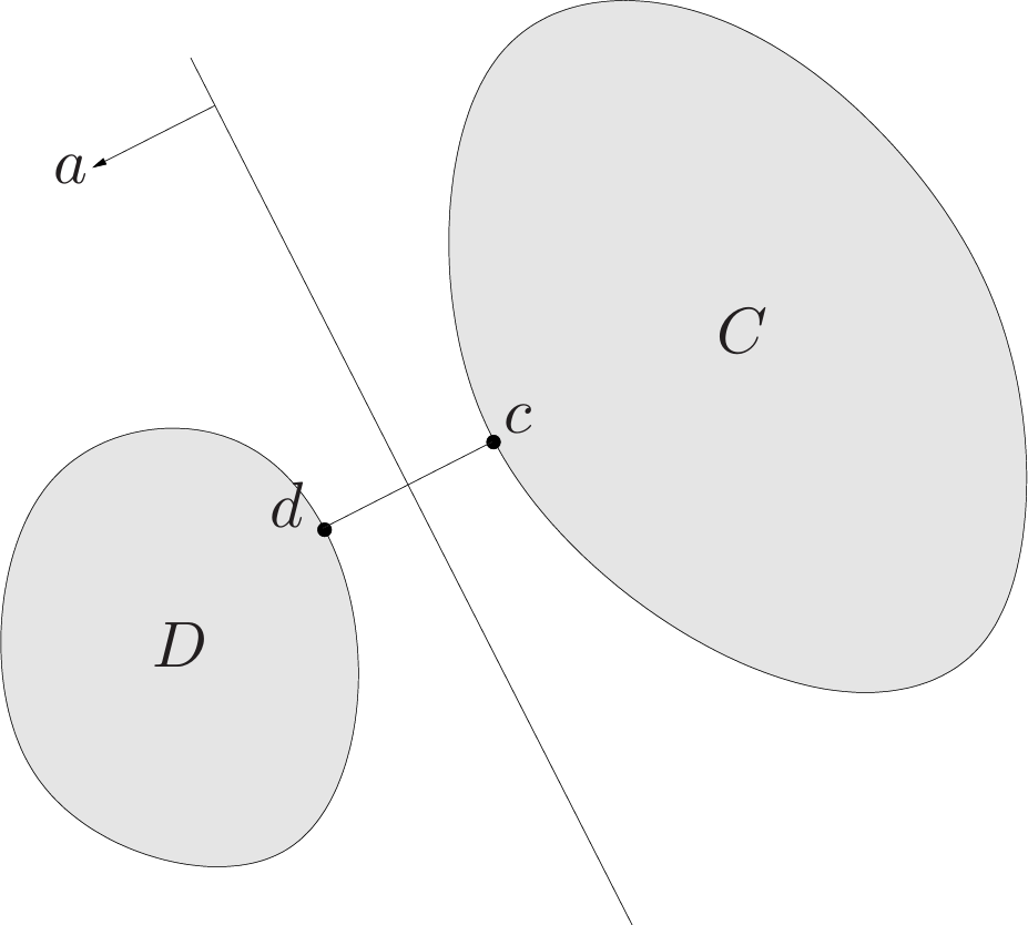
Here we consider a special case, we assume that the (Euclidean) distance between $C$ and $D$, defined as

$$\begin{gathered} \mathbf{dist}(C,D)=\text{inf} \\ \Vert u-v{\Vert }_2|u\in C,v\in D \end{gathered}$$

is positive, and that there exist points $c\in C$ and $d\in D$ that achieve the minimum distance, i.e., $\Vert c-d{\Vert }_2=\mathbf{dist}(C,D)$. (These conditions are satisfied, for example, when $C$ and $D$ are closed and one set is bounded.)

Define

$$a=d-c,b=\frac{\Vert d{\Vert }_2^2-\Vert c{\Vert }_2^2}{2}$$

We will show that the affine function

$$f(x)=a^{T}x-b=(d-c{)}^T(x-(1/2)(d+c))$$

is nonpositive on $C$ and nonnegative on $D$, i.e., that the hyperplane $\{x

a^Tx=b\}$separates$C$and$D$.

This hyperplane is perpendicular to the line segment between $c$ and $d$, and passes through its midpoint.

We first show that $f$ is nonnegative on $D$. The proof that $f$ is nonpositive on $C$ is similar (or follows by swapping $C$ and $D$ and considering $-f$). Suppose there were a point $u\in D$ for which

$$f(u)=(d-c{)}^T(u-(1/2)(d+c))<0$$

We can express $f(u)$ as

$$f(u)=(d-c{)}^T(u-d+(1/2)(d-c))=(d-c{)}^T(u-d)+(1/2)\Vert d-c{\Vert }_2^2$$

We see that $(d-c{)}^T(u-d)<0$. Now we observe that

$$\frac{d}{dt}\Vert d+t(u-d)-c{\Vert }_2^2{|}_{t=0}=2(d-c{)}^T(u-d)<0$$

so for some small $t>0$, with $t\le 1$, we have

$$\Vert d+t(u-d)-c{\Vert }_2<\Vert d-c{\Vert }_2$$

i.e., the point $d+t(u-d)$ is closer to $c$ than $d$ is. Since $D$ is convex and contains $d$ and $u$, we have $d+t(u-d)\in D$. But this is impossible, since $d$ is assumed to be the point in $D$ that is closest to $C$.

Strict separation:

The separation hyperplane we constructed above satisfies the stronger condition that $a^{T}x<b$ for all $x\in C$ and $a^{T}x>b$ for all $x\in D$. This is called strict separation of the sets $C$ and $D$.

Converse separating hyperplane theorems:

Any two convex sets $C$ and $D$, at least one of which is open, are disjoint if and only if there exists a separating hyperplane.

2.5.2 Supporting hyperplanes

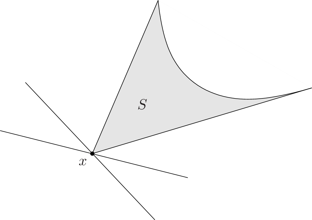
Suppose $C\in {\mathbf{R}}^n$, and $x_0$ is a point in its boundary $\mathbf{bd}C$, i.e.,

$$x_0\in \mathbf{bd}C=\mathbf{cl}C\mathrm{\setminus }\mathbf{int}C$$

If $a\ne 0$ satisfies $a^{T}x\le a^T{x}_0$ for all $x\in C$, then the hyperplane $\{x

a^Tx=a^Tx_0\}$ is called a supporting hyperplane to $C$ at the point $x_0$. This is equivalent to saying that the point $x_0$ and the set $C$ are separated by the hyperplane $\{x

a^Tx=a^Tx_0\}$.Thegeometricinterpretationisthatthehyperplane$\{x

a^Tx=a^Tx_0\}$istangentto$C$at$x_0$,andthehalfspace$\{x

a^Tx\leq a^Tx_0\}$contains$C$.

![Fig. 2. The hyperplane ${x

a^Tx=a^Tx_0}$supports$C$at$x_0$](/assets/images/2024-02-12-convex-optimization-chapter2/2024-02-11-09-30-17.png)

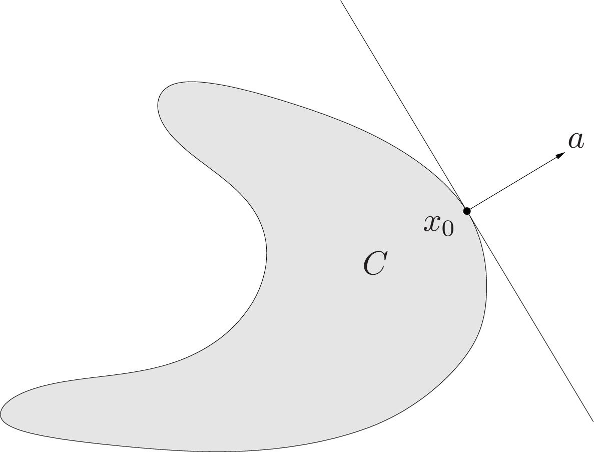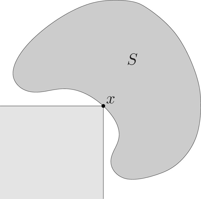
A basic result, called the supporting hyperplane theorem, states that for any nonempty convex set $C$, and any $x_0\in \mathbf{bd}C$, there exists a supporting hyperplane to $C$ at $x_0$.

There is also a partial converse of the supporting hyperplane theorem: If a set is closed, has nonempty interior, and has a supporting hyperplane at every point in its boundary, then it is convex.

2.6 Dual cones and generalized inequalities

2.6.1 Dual cones

Let $K$ be a cone. The set

$$\begin{gathered} K^{\ast }= \\ y|x^{T}y\ge 0\text{ for all }x\in K \end{gathered}$$

is called the dual cone of $K$. As the name suggests, $K^{\ast }$ is a cone, and is always convex, even when the original cone $K$ is not.

Geometrically, $y\in K^{\ast }$ if and only if $-y$ is the normal of a hyperplane that supports $K$ at the origin.

Subspace. The dual cone of a subspace $V\subseteq {\mathbf{R}}^n$ (which is a cone) is its orthogonal complement $V^{\perp}=\{y

v^Ty=0\text{ for all }v\in V\}$.

Nonnegative orthant. The cone ${\mathbf{R}}_{+}^n$ is its own dual:

$$x^{T}y\ge 0\text{ for all }x⪰0\iff y⪰0$$

We call such a cone self-dual.

Duyal cones satisfy several properties, such as:

• $K^{\ast }$ is closed and convex.
• $K_1\subseteq K_2$ implies $K_2^{\ast }\subseteq K_1^{\ast }$.
• If $K$ has nonempty interior, then $K^{\ast }$ is pointed.
• If the closure of $K$ is pointed then $K^{\ast }$ has nonempty interior.
• $K^{\ast \ast }$ is the closure of the convex hull of $K$. (Hence if $K$ is convex and closed, $K^{\ast \ast }=K$.)

These properties show that if $K$ is a proper cone, then so is its dual $K^{\ast }$, and moreover, that $K^{\ast \ast }=K$.

2.6.2 Dual generalized inequalities

Now suppose that the convex cone $K$ is proper, so it induces a generalized inequality ${⪯}_K$. Then its dual cone $K^{\ast }$ is also proper, and therefore induces a generalized inequality. We refer to the generalized inequality ${⪯}_{K^{\ast }}$ as the dual of the generalized inequality ${⪯}_K$.

Some important properties relating a generalized inequality and its dual are:

• $x{⪯}_{K}y$ if and only if ${\lambda }^{T}v\le {\lambda }^{T}y$ for all $\lambda {⪰}_{K^{\ast }}0$.
• $x{\prec }_{K}y$ if and only if ${\lambda }^{T}v<{\lambda }^{T}y$ for all $\lambda {⪰}_{K^{\ast }}0,\lambda \ne 0$.

Since $K=K^{\ast \ast }$, the dual generalized inequality associated with ${⪯}_{K^{\ast }}$ is ${⪯}_K$, so these properties hold if the generalized inequality and its dual are swapped. As a specific example, we have $\lambda {⪯}_{K\ast }\mu$ if and only if ${\lambda }^{T}x\le {\mu }^{T}x$ for all $x{⪰}_{K}0$.

2.6.3 Minimum and minimal elements via dual inequalities

Dual characterization of minimum element:

We first consider a characterization of the minimum element: $x$ is the minimum element of $S$, with respect to the generalized inequality ${⪰}_K$, if and only if for all $\lambda {\prec }_{K\ast }0$,$x$ is the unique minimizer of ${\lambda }^{T}x$ over $z\in S$. Geometrically, this means that for any $\lambda {\prec }_{K\ast }0$, the hyperplane

$$z|{\lambda }^T(z-x)=0$$

is a strict support hyperplane to $S$ at $x$. Note that convexity of the set $S$ is not required.

Dual characterization of minimal element:

We now turn to a similar characterization of minimal elements. Here there is a gap between the necessary and sufficient conditions. If $\lambda {\prec }_{K\ast }0$ and $x$ minimizes ${\lambda }^{T}z$ over $z\in S$, then $x$ is minimal.

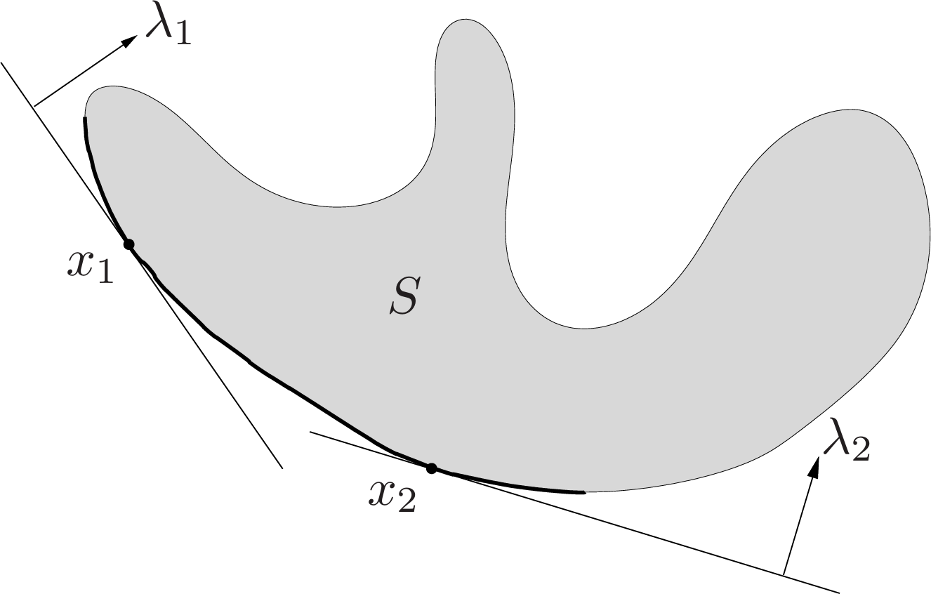
The converse is in general false: a point $x$ can be minimal in $S$, but not a minimizer of ${\lambda }^{T}z$ over $z\in S$, for any $\lambda$.

Provided the set $S$ is convex, we can say that for any minimal element $x$ there exists a nonzero $\lambda {⪰}_{K^{\ast }}0$ such that $x$ minimizes ${\lambda }^{T}z$ over $z\in S$.

This converse theorem cannot be strengthened to $\lambda {\succ }_{K\ast }0$.